Split by Delimiter into Rows (and Columns) with Power Query

12/1/2020

Bottom Line: Learn how to use the Split by Delimiter into Rows and Columns features of Power Query. Also see how to trim blank spaces and replace values. 

Skill Level: Intermediate

Convert a Block of Email Addresses to an Organized List

Let's say you've just joined a new group (distribution list) and you want to make a list or directory of the members' contact information. The data that you have to start your list is from a group email that you received.

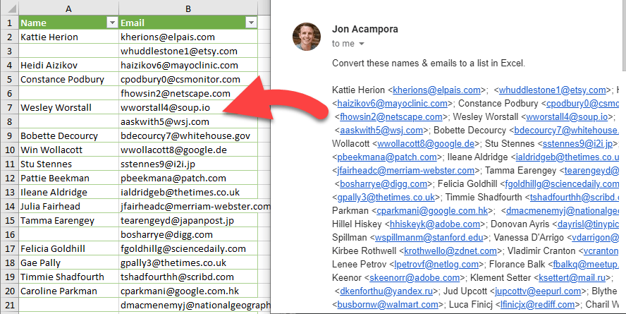
You can take the string of names and emails in the “To” field of your email and quickly turn them into an organized list using Power Query. I'll show you how to turn the data on the right into a table like the one on the left.

Using Power Query to Create a Table

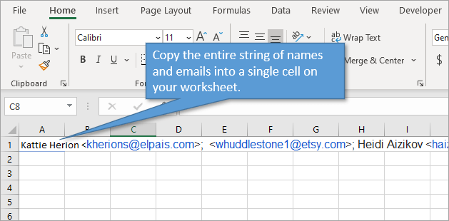
The first step in transforming our data is just to copy the entire block, or string, of names/emails. Then paste them into one cell on an Excel worksheet.

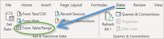
With that one cell selected, open up the Power Query Editor. You can do that by clicking on From Table/Range on the Data tab of the Ribbon.

That will bring up the Create Table window. Verify the cell that you are pulling the data from, and that the checkbox for “My table has headers” is NOT checked. When you click OK, the Power Query Editor will open.

1. Split by Delimiter into Rows

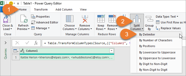
The first thing we are going to do in the editor is split our column. On the Home tab of the Ribbon, go to the Split Column menu and choose By Delimiter.

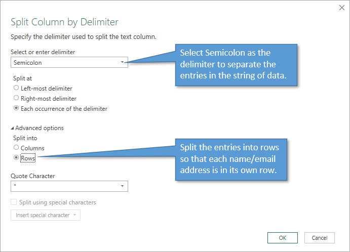
A delimiter is a character, symbol, or space that indicates the beginning or end of a data item. In our case, our email entries are separated from each other by a semicolon. So when the Split Column by Delimiter window appears, select Semicolon from the dropdown menu of delimiters.

In the same window, under Advanced Options, select the option for splitting into Rows. Otherwise each of our email entries will be listed in its own column, which isn't helpful for us.

When you kit OK, your data string will be split so that each row contains the data that was formerly between semicolons.

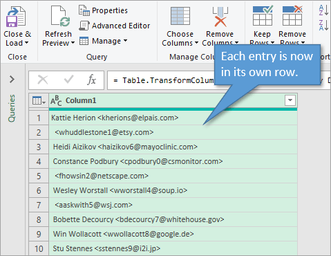
This is an awesome and somewhat hidden feature of Power Query! And it still works the same if your data table has multiple columns but you are only splitting a single column.

2. Split by Delimiter into Columns

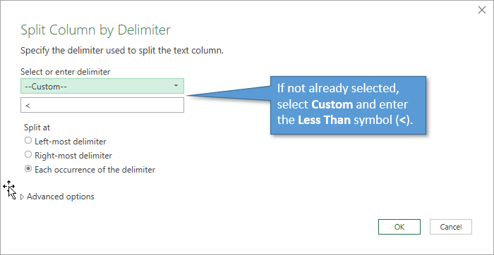
Our next step is to separate the names from the email addresses. What symbol separates these pieces of data? The less than symbol (<). So we will repeat the process of splitting by delimiter, but this time we will choose the less than symbol, which can be typed in when you choose the Custom option for your delimiter. Don't select the Advanced Option for Rows this time. We want our data to be split into columns.

Here's what the data looks like now.

Cleaning Up the Data

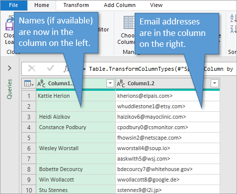
Next we have a bit of data cleansing work to do.

1. Remove Blank Spaces with Trim

You'll notice that in the first column, there are extra spaces before the names. To get rid of those, just right-click on the column header and select Transform, then Trim.

2. Remove Extra Characters with Replace Values

In the second column, we want to get rid of the greater than symbols (>) that follow each email address. To do that, right-click on the column header, select Replace Values, and then replace the > with nothing. This will remove all of those marks.

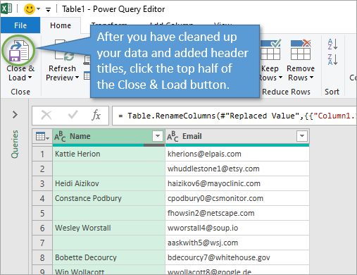
And finally, we want to add column header titles. To do that, double-click the header for each column and type in the new name. (In our case, Column 1 becomes Name and Column 2 becomes Email.)

3. Rename the Columns

Finally, we can double-click each column header and give the columns descriptive names.

Output the Query to an Excel Table

Now click on the top half of the Close & Load button. This exports the data out of Power Query into its own new worksheet.

Your new worksheet lists each of the names and email addresses in their own cells of an organized table.

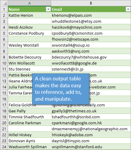
Using Power Query, we've split the data using delimiters, first into rows so each email/name has its own entry, then by columns so the name is separated from the email address.

A Fully Automated Process

Because we built this process in Power Query, we are able to reuse it. Any new list of emails that comes in can be cleaned up quickly now that we've done the work of setting it up.

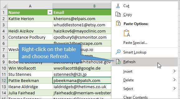
To do that, you can just paste the new list into the cell that had the original list and rerun the query, which is really simple to do. Just right-click anywhere on the output table and choose Refresh.

Or if you are looking to add new entries to your existing output table, you can simply paste the data into the next empty cell in the source column. In the image below, I've pasted the first list of emails into A2 and the second list into A3.

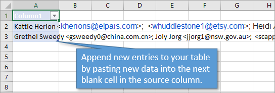
This set-up will append the second list to the first list when you refresh the output table. Append means stacking the data; the second list will be put below the first list in the output table.

Source: excelcampus.com