How to Create Icons with Conditional Formatting in Excel

3/18/2020

Bottom Line: Learn a technique for applying conditional formatting to the new icons in Excel.

Skill Level: Intermediate

Specially Formatted Icons

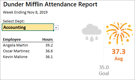
For our final task in creating the attendance dashboard, we want to create icons that change depending on departmental performance. Specifically, when a department exceeds its attendance goal, a firework icon will be colored while the storm cloud icon is grayed out.

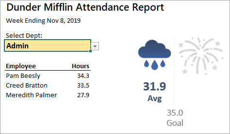
And conversely, when the department does not meet its goal, the storm cloud is colored and the firework is gray.

Selecting Icons

To find the icons you want, you can use the new Icons window, which has a search feature. To access this window, go to the Insert tab on the Ribbon. Select Illustrations, and then Icons.

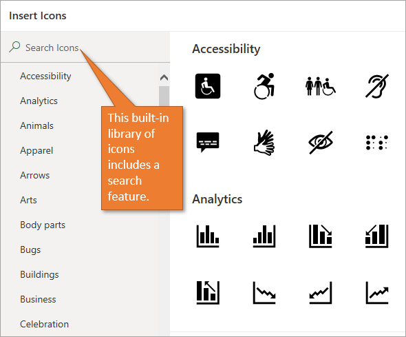
Select the icons you want to insert. (You can insert more than one at a time.)

Formatting Your Images

We're going to change our icons to a picture by making some alterations to it. Start by changing the color of the icons to a very light gray. You can do this by selecting Graphics Fill on the Graphics Format tab on the Ribbon.

Next, insert a white square, which will be the background to your icon. You can insert this square by going to the Insert tab on the Ribbon, choosing the Illustrations button, and selecting Shapes. You'll get a menu of shapes to choose from, and you can select a rectangular shape.

Draw the square around the icon and change the Shape Fill to white. Change the Shape Outline setting to No Outline. Then right-click on the shape and choose Send to Back from the menu that appears. That places a white background behind your icon.

With the background shape selected, hold the Ctrl button on the keyboard and select the icon as well. Then right-click and choose Group to group the two shapes together.

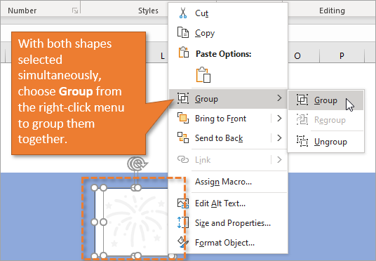
Copy this new group and then paste it elsewhere on the sheet. But don't do a normal paste. Right-click and choose Paste Options, then Picture. What this does is it takes that group of two shapes and makes it into one image.

With your new image selected, go to the Picture Format tab on the Ribbon and select the Color option. Near the bottom of that menu is Set Transparent Color.

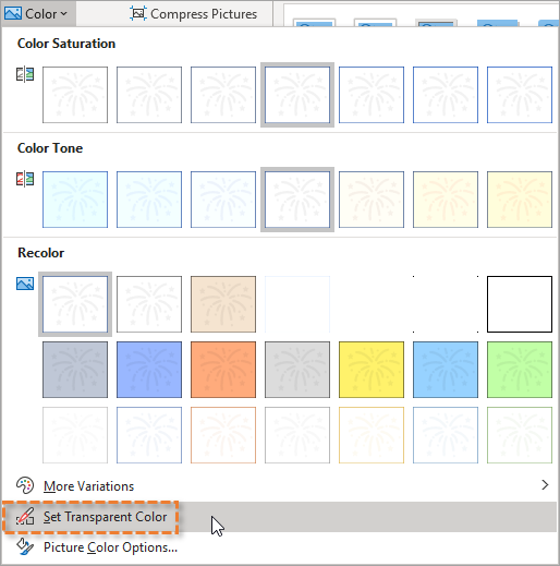
This changes your mouse cursor so that whatever you click on next will have a transparent fill. In other words, it will be clear instead of colored.

You'll want to repeat all of that formatting for your second icon as well.

Conditional Formatting

Now that we have icons you can see through, we are going to set them on specific cells that we can reference in our conditional formatting.

From the Home tab, you can select Conditional Formatting and choose Manage Rules. This pulls up the Conditional Formatting Rules Manager. I've set rules for both of the cells that have icons in them.

One of the rules fills the storm cloud with a gradient blue if the actual attendance number is lower than the target number. The other rule fills the firework with a gradient orange color if the actual is higher than the target. If the conditions are not met to format them in these ways, the icon color will be just a light gray instead.

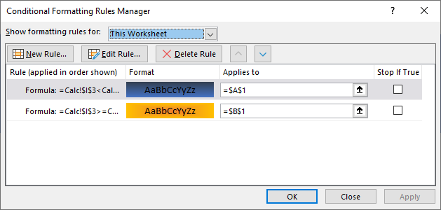
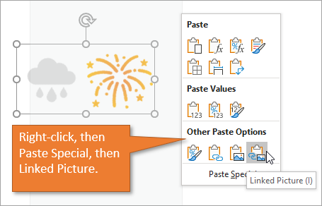
Now that we have created our conditional formatting rules for those two cells, we can copy and paste them onto the Dashboard sheet. When we paste, we want to Paste Special as a Linked Picture.

Adding Text Boxes

Lastly, we are going to add text boxes, below each icon, that are also conditional. These text boxes will display a number or remain blank depending on if the the department average is higher or lower than the overall goal. That's because these text boxes are linked to the cell on the Calc sheet that has the IF formula that spells out those conditions.

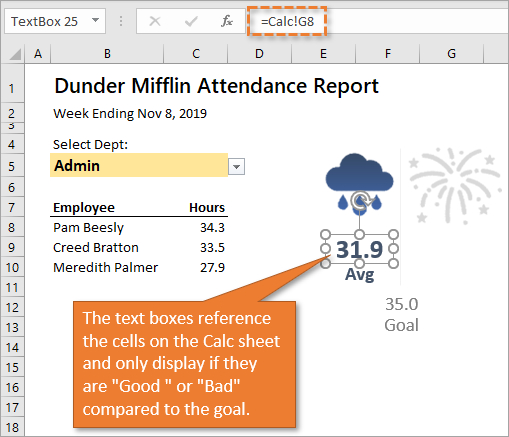
Adding the text boxes is easily done. Just go to the Insert tab on the Ribbon and click on the Text button, and select Text Box. You can then draw the text box on the worksheet with your mouse.

To link the text box, just click on it, type the equals sign (=) in the formula bar, and select the cell on the Calc sheet that you want to link it to. You can format the text box however you like.

Source: Excel Campus