How to Create a Pivot Table using Multiple Files in Excel

5/7/2020

Sometimes we receive or capture our data in different workbooks and in that case creating a pivot table need some extra efforts for combining those multiple workbooks into one.

Only after that, we can create a pivot table.

So in this post, I’d like to show you a 3 steps process to create a pivot table by using data from multiple workbooks.

So let’s get started.

Steps to Create a Pivot Table using Data from Multiple Workbooks

 Important: For this, we need to use power query.

Make sure you have power query in your Excel version. For Excel 2016, it’s there on the Data tab and for other versions (2010 and 2013) you need to install the add-on.

 

Here I have four different workbooks with sales data for different zones. You can download these files from here to follow along.

And make sure you have all these files in a single folder.

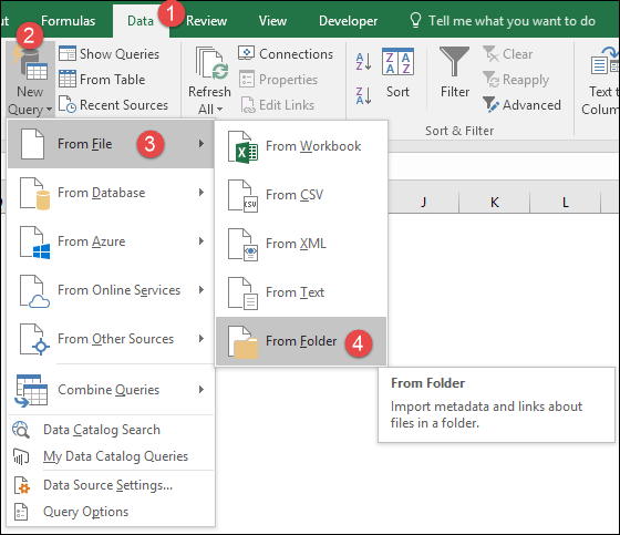
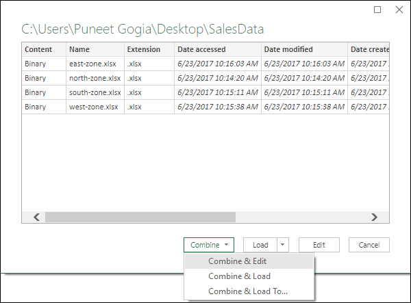
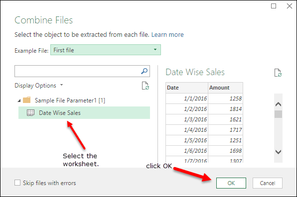
Step 1 - Combine Files using Power Query

First of all, we need to combine all the files into one file with power query.

• Go to Data Tab -> Get Transformation -> New Query -> From File -> From Folder.

• Now, from the folder selection window, click on “Browse” and select the folder where you have all the files.

• Click OK.
• From here, you’ll get a “Combine Files” window.

• And from that window, select the worksheet in with you data in all the workbooks. (Quick Tip: Make sure to have the same worksheet name in all the workbooks).

• Once you click OK and it will edit all the data from the workbooks into power query editor.

Step 2 - Prepare Data for the Pivot Table

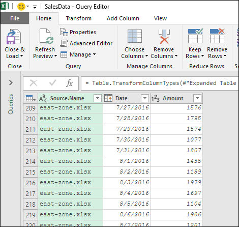
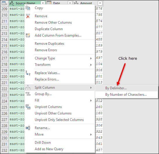
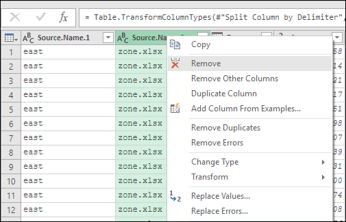
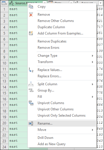
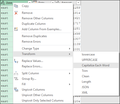
Now, we need to make little changes in our data to make it ready for a pivot table.

• If you look at the data we have got an extra column here with the name of the source file.

• Right click on this column and select Split Column -> By Delimiter.

• From delimiter window, select custom, add “-” as a delimiter, and select “Left-most delimiter”.

• Click OK.

• After that, delete the second column.

• Now, rename the first column.

• One more thing, right-click on the first column again and go to Transform -> Capitalize Each Word.

• And, now your data is ready. So, click on close and load.

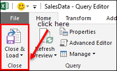
Step 3 - Insert the Pivot Table

At this point, we have a new worksheet in our workbook with the combine data from all the four files.

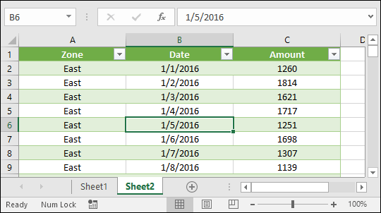
Now, it’s time to create a pivot table from it.

• Select the table and go to Insert Tab and click on the Pivot Table button.

• Here you’ll get an insert pivot table window.

• Click OK on insert pivot table window and you’ll get new pivot table in your workbook.

 

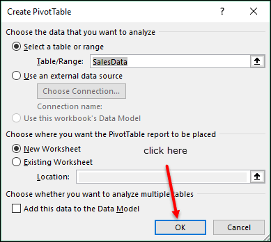
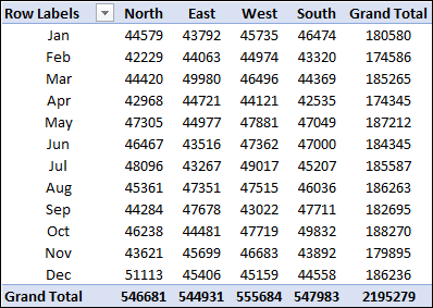
Refresh Pivot Table

I’m sure you are thinking about how to refresh your pivot table after updating source files.

It’s simple.

To refresh your pivot table you need to update the query so that the data from the source file can be updated in the source table which you created with power query. And after that, you can update your pivot table.

But, the simple and best way is to use refresh button from the data tab. It will refersh both (Pivot Table + Query).

Important Points

Here I have listed some points which you need to remember while using power query for a pivot table.

• Files should be in a single folder.
• Data should be in the same format in all the files. Otherwise, you need to make it usable after combining from it.
• Name of the worksheets should be same in all the files.
• Make sure you don’t have any error in any file. Or you can use “Skip error files” option.
• Don’t rename any workbook.