How to Compare Two Columns in Excel

6/30/2021

How to Compare Two Columns in Excel

Suppose you have two lists of students' names in Column A and Column B of your worksheet, and some of them are in two columns, but, you want to compare these two columns and insert the different names from them.

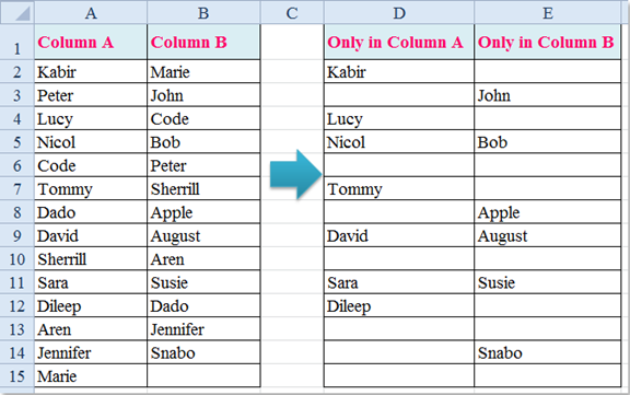
To list unique values from the two lists separately, you can apply the following formulas:

1. Enter this formula in cell D2: =IF((ISERROR(MATCH(A2,$B$2:$B$14,0,2))),AXNUMX,“”), (A2 is the first cell inside column A that you want to compare with column B and range $2:$14 refers to another column you want to compare) and then press the Enter key:

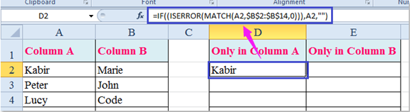
2. Drag the fill handle down to the cells that you want to apply this formula, and all the unique names in column A are only inserted once:

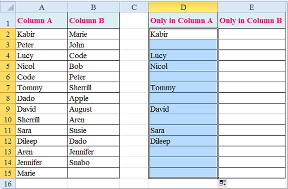
3. Keep entering this formula: =IF((ISERROR(MATCH(B2,$A$2:$15,0,2))),BXNUMX,“”) into cell E2, and press Enter key:

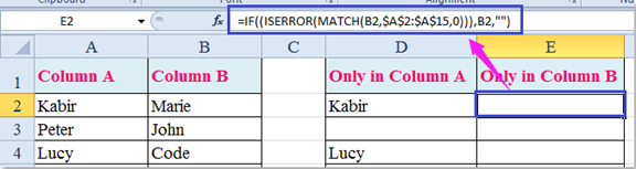
4. Select cell E2, and drag the fill handle to the cells that you want to contain this formula, after which all the names in column B have been extracted only as follows:

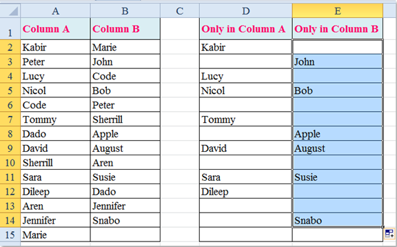
Now all the unique names in both columns are listed.

Compare Two Columns, Row by Row

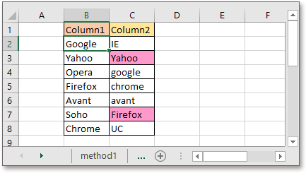
Below is a dataset where I need to check in the same row whether or not the names in column A match those in column B.

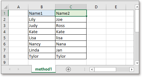
Compare Cells in the Same Row to Get an Exact Match

Usually, if you want to compare two columns row by row for an exact match, you can use the following formula: =B2=C2

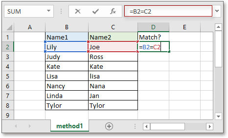
Press the Enter key and drag the fill handle down to cell D8. If the formula returns TRUE, then the two-column values are precisely the same; if it returns FALSE, they are different.

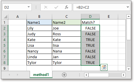
Compare Cells in the Same Row for Exact Matches or Case Insensitive (Using the IF formula)

If you want to compare two columns row by row in insensitive characters or get more descriptions such as match, mismatch, you can use the IF function.

Compare cells in the same row for an exact match

If you want to use the text “Match” and “Mismatch” to describe the results of the comparison, please use the following formula: =IF(EXACT(B2, C2),“Match”,“Mismatch”)

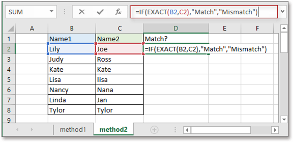
Press the Enter key to get the first result, then drag the AutoFill handle to cell D8.

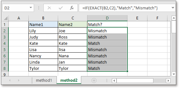
Compare Cells in the Same Row for a Case-Insensitive Match

If you want to compare cells that are not case sensitive, you can use the formula below: =IF(B2=C2,"Match","Mismatch")

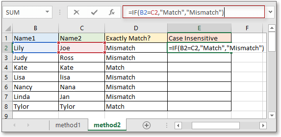
Press the Enter key to get the first result, then drag the AutoFill handle to cell E8.

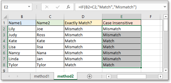
Compare Cells in the Same Row and Highlight Matching or Unmatched Data (Using Conditional Formatting)

If you want to distinguish matching or different values, the Conditional Format file feature can help you.

1. Select the two columns used for comparison (B2:C8, excluding column headers), then click Home> Conditional Formatting> New Rule.

2. In the New Format Rule appeared dialog, click to use a formula to specify the cells to format in the Select a rule type, then type =$B2=$C2 in the Format Values text box formula is correct.

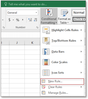
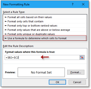
3. Now, click a shape to display the Format Cells dialog, then under the Run tab, choose one color that you want to highlight matches.

Or, you can change the font size, font size, cell boundaries, or number format to beat matches as you want on other tabs.

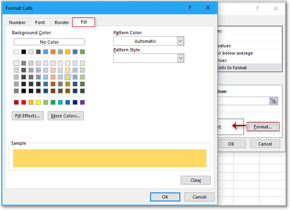
 4. Click OK to close the dialog boxes; the cells in the same row will be selected if they are identical.

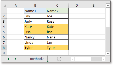
If you want to highlight mismatch values, you can use =$B2<>$C2 in the textbox values format where this formula is correct in the Edit Formatting Rule dialog.

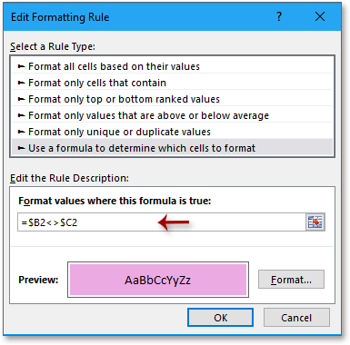
Then the differences between two columns in the same row will be highlighted with a specific color.

Compare Two Columns Row by Row and Mark Mismatch Values (using VBA)

This tutorial is for you if you want to compare two columns row by row with VBA code.

1. Enable the Worksheet containing the two columns used for comparison, press the ALT + F11 keys to enable the Microsoft Visual Basic for Applications window.
2. In the popping dialog, click Insert> Module.

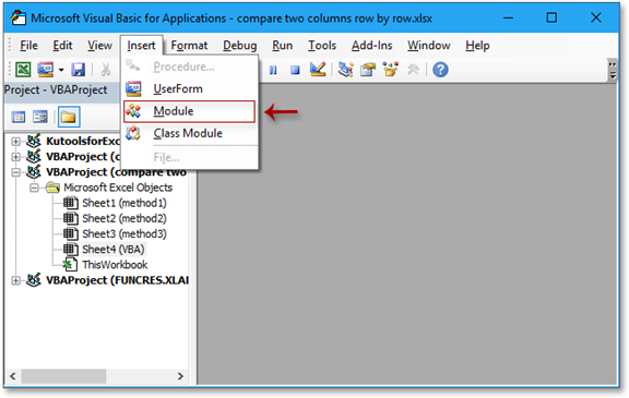
Then copy and paste the macro below into the new module script.

• Sub ExtendOffice_HighlightColumnDifferences()
• 'UpdatebyKutools20201016
• Dim xRg As Range
• Dim xWs As Worksheet
• Dim xFI As Integer
• On Error Resume Next
• SRg:
• Set xRg = Application.InputBox("Select two columns:", "Kutools for Excel", , , , , , 8)
• If xRg Is Nothing Then Exit Sub
• If xRg.Columns.Count <> 2 Then
• MsgBox "Please select two columns"
• GoTo SRg
• End If
• Set xWs = xRg.Worksheet
• For xFI = 1 To xRg.Rows.Count
• If Not StrComp(xRg.Cells(xFI, 1), xRg.Cells(xFI, 2), vbBinaryCompare) = 0 Then
• Range(xRg.Cells(xFI, 1), xRg.Cells(xFI, 2)).Interior.ColorIndex = 7 'you can change the color index as you need.
• End If
• Next xFI
• End Sub

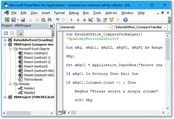
Press the F5 key to run the code. In the first pop-up dialog, select the column against which you want to compare duplicate values.

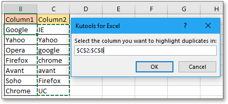
Click OK. In the second dialog box, select the column in which you want duplicate values highlighted.

• The code compares the columns with case sensitivity.
• You can change the shading color based on your unique need by changing the color index in the code, color index reference:

Source: www.simplesheets.co