3 tips to save time when working with the Pivot Table Field List

7/15/2021

The Pivot Table Task Pane

When working with pivot tables, there's is a task pane that is used to add or delete fields to different areas of the table. This is the Pivot Table Fields list and I'd like to share with you three tips to help you use it more efficiently. 

Tip #1: Change the Layout of the Field List

The first tip involves modifying how the pane is laid out. The default layout of this pane is as shown above, with the fields listed on top and the areas underneath. But the layout can be changed to a few other configurations. To change the layout, simply click on the settings dropdown menu. It's the button that has the gear icon on it. 

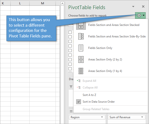
Of the alternate layouts that are offered, I think I prefer the side-by-side layout most. That's because it allows for more fields to be shown in list form without scrolling, which is really helpful when there are many fields to choose from. 

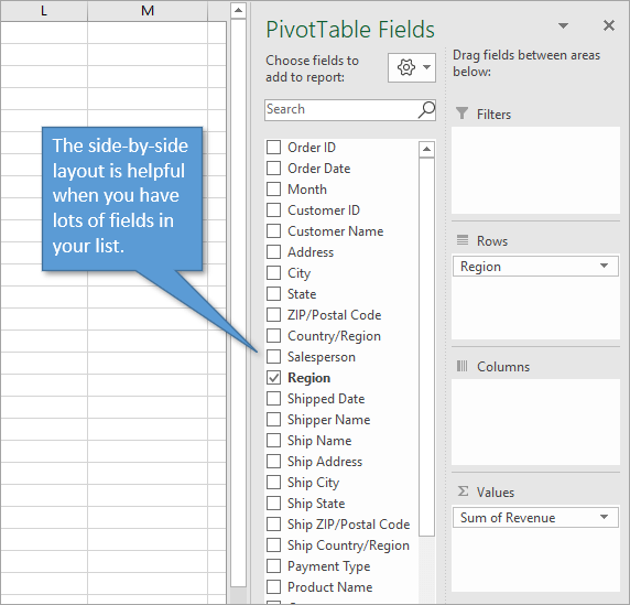
This layout is also helpful when you are using Power Pivot. Other layout options that are less popular, but still useful, are fields only, areas only, and and stacked areas only. 

Other Features in the Settings Menu

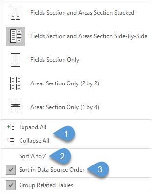
In addition to changing the layout of the pane, the settings menu allows you to do a few more things as well:

1. If you are using Power Pivot, you can collapse and expand the table fields.

2. You can sort the fields in alphabetical order.

3. You can sort in data source order. (This would be the columns in your data set, from left to right).

Tip #2: Undock and Move the Fields List

By default, the fields list is docked to the right of your worksheet. But you can move it. Hover your cursor near the title of the pane until it turns into a cross-arrows. Then left-click and drag the pane to your desired location. 

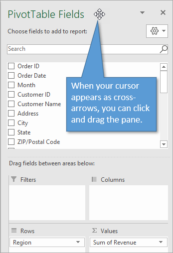
Once the pane has been undocked, you are able to resize it as you like. You can also dock the pane to the left side of the worksheet as well. If the pane is floating, you can double-click the top to instantly redock it to whichever side it was last docked at. 

One other feature to note is that you can move the pane off of the application completely. So if you have multiple monitors, for example, you could have the worksheet on one monitor and the fields list on another monitor. 

Tip #3: Reopening the Fields List When Closed

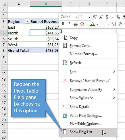
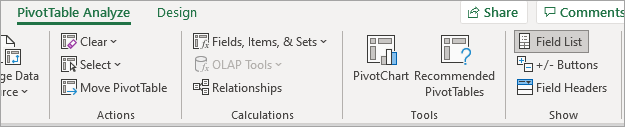
Sometimes you might inadvertently make the Pivot Table Fields list disappear. Or you may close it purposely but not be aware of how to get it back. If you've closed the window, clicking anywhere in the pivot table will NOT bring it back. Instead you can reopen it in one of two ways. 

1. Right-click on the pivot table and then select Show Field List. 

2. Click the Field List button on the PivotTable Analyze or Options tab.

Bonus Tip: Managing Multiple Task Panes

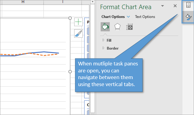
One other tip I want to mention concerns having multiple task panes open simultaneously. In the image below, you can see that I have the Format Chart Area task pane open, and it has eclipsed my Pivot Table Fields pane. To navigate between the two, click on the icons that are aligned vertically down the right side of the pane. The top icon indicates the Pivot Chart Fields pane and the bottom one is the Format Chart Area pane. If I had more panes open, they would appear below these as vertical tabs. 

Source: www.excelcampus.com